Quantum Machine Learning
Quantum Machine Learning Project
Statement of Collaboration: I undertook this project in college with three other students: Gabe Apoj, Tomislav Zabcic-Matic, and Sean Murphy. Having taught machine learning and quantum computing classes, I am pleased that this project remains relevant four years later. To showcase and explain some of our work, I am now going back and writing a report.
§ 1Quantum Machine Learning
There is a high motivation to apply the theoretical efficiency boost of quantum computing to machine learning. The impact of machine learning is directly proportional to the amount of computing and data placed behind it. GPT-3 (and therefore Chat-GPT which was later derived from it) took an estimated 1.287 gigawatt-hours of energy and $5 Million to full train.
We, therefore, turned our attention to Maria Schuld, a leader in the quantum machine learning space, and decided to base our project on her distance-based binary classification paper:
Implementing a distance-based classifier with a quantum interference circuit
Until now, most papers focused on taking a typical machine-learning algorithm and simply porting it onto a quantum computer.
"Most importantly, quantum machine learning remains an enterprise to merely mimic methods from classical machine learning that have been tailor-made for classical computation." - Schuld et al.
I should note trying to get classical algorithms to run on a quantum computer is not a trivial process; you have neither the bandwidth nor the tools necessary to implement them easily. However, what made Schuld et al.'s paper stand out was that they desired to emulate the act of classifying using the most native quantum way possible:
"Instead of choosing a textbook machine learning algorithm and asking how to run it on a quantum computer, we turn the question around and ask what classifier can be realized by a minimum quantum circuit." - Schuld et al.
We had the unique opportunity to work with two completely different superconducting quantum device architectures: The Rigetti Aspen-4 16-qubit device, and the IBMQ Tenerife 5-qubit device.
Our goal for this project was, therefore, twofold:
- Implement the theoretical classifier proposed by Schuld et al. in both IBM and Rigetti quantum programming languages.
- Test the classifier's performance on both quantum systems on the same Iris dataset.
§ 2Method
The Iris dataset, a true classic, has four feature dimensions and three classes to classify:
Sepal: Length, width
Petal: Length, width
Flower Variety: Versicolor, Setosa, Virginica
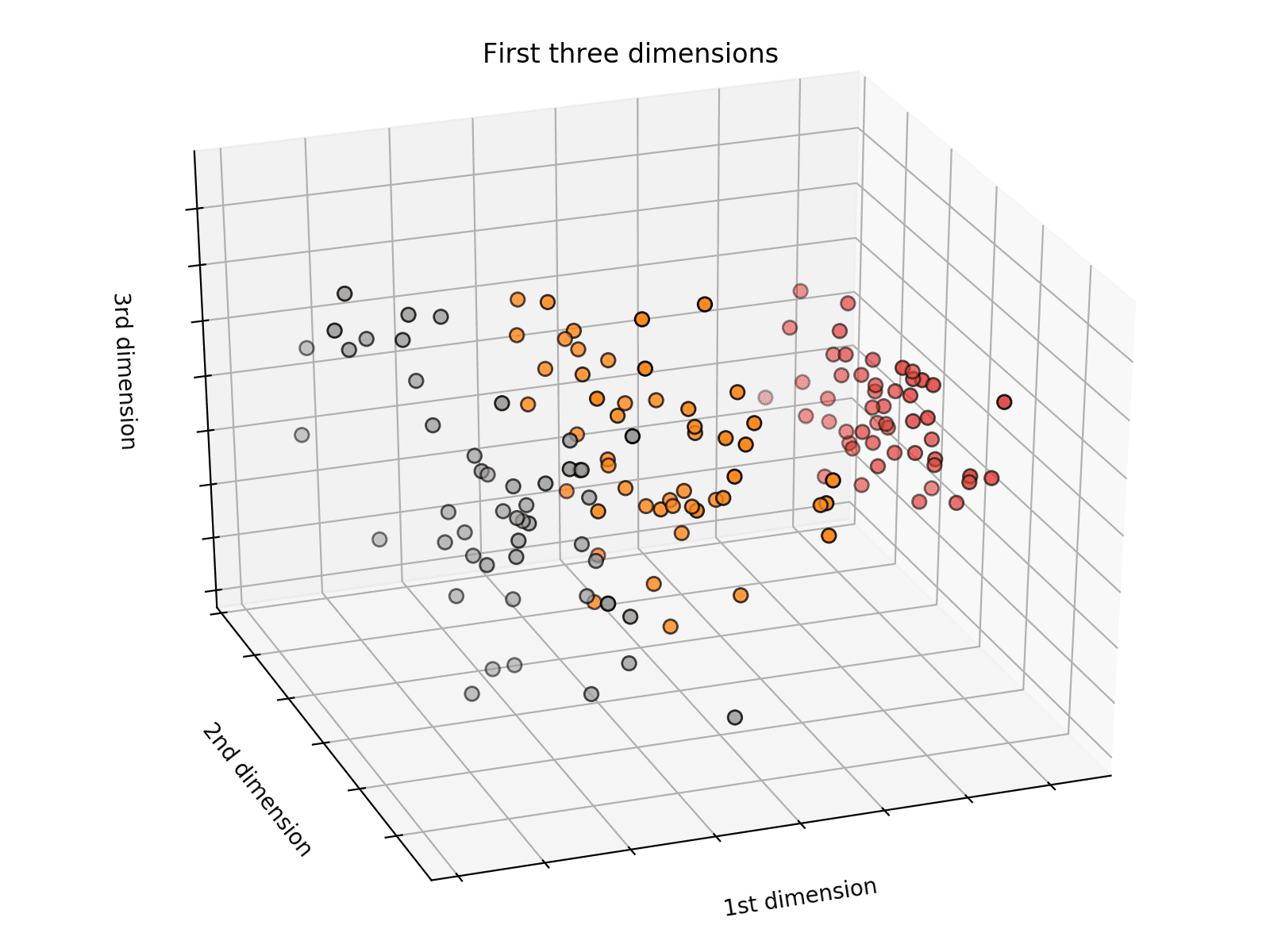
Here we are visualizing only three of the four feature dimensions, showing each flower in grey, orange, and red, respectively. The diagram indicates that two of the three flower types are easier to distinguish than the other. The gray and red classes are linearly separable and, therefore, easier to classify than the orange ones.
Making the Quantum Circuit
We constructed the following quantum circuit as similarly as possible in Qiskit and PyQuil for each quantum device, respectively. Note how both circuits are parameterized versions of this example diagram, taking in a two-dimensional angles parameter.
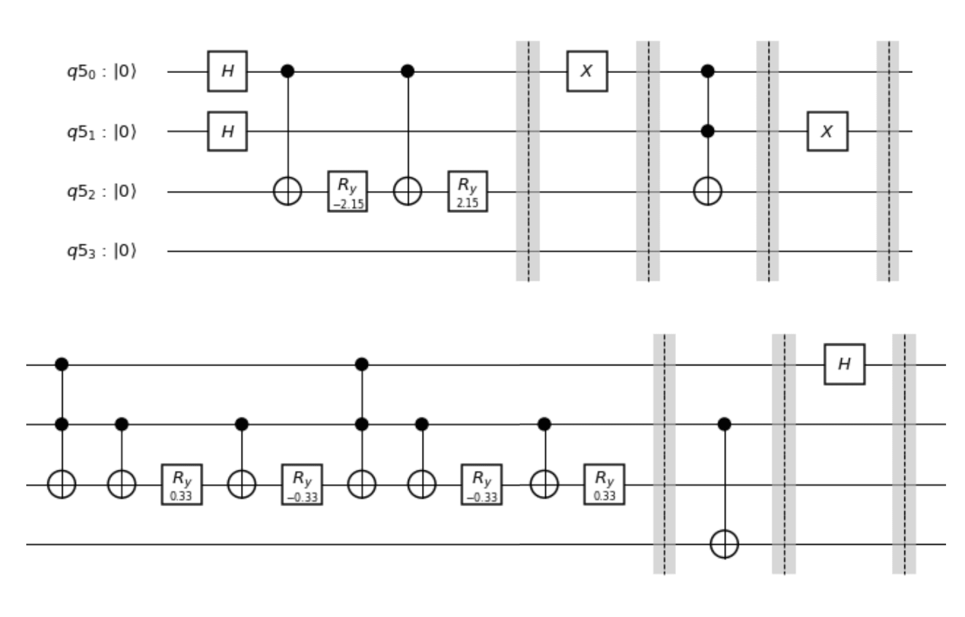
Qiskit Quantum Circuit
pythondef create_circuit(self, angles):
  qc = QuantumCircuit(self.q, self.c)
  qc.h(self.ancilla_qubit)
  qc.h(self.index_qubit)
  qc.cx(self.ancilla_qubit, self.data_qubit)
  qc.u3(-angles[0], 0, 0, self.data_qubit)
  qc.cx(self.ancilla_qubit, self.data_qubit)
  qc.u3(angles[0], 0, 0, self.data_qubit)
  qc.barrier()
  qc.x(self.ancilla_qubit)
  qc.barrier()
  qc.ccx(self.ancilla_qubit, self.index_qubit, self.data_qubit)
  qc.barrier()
  qc.x(self.index_qubit)
  qc.barrier()
  qc.ccx(self.ancilla_qubit, self.index_qubit, self.data_qubit)
  qc.cx(self.index_qubit, self.data_qubit)
  qc.u3(angles[1], 0, 0, self.data_qubit)
  qc.cx(self.index_qubit, self.data_qubit)
  qc.u3(-angles[1], 0, 0, self.data_qubit)
  qc.ccx(self.ancilla_qubit, self.index_qubit, self.data_qubit)
  qc.cx(self.index_qubit, self.data_qubit)
  qc.u3(-angles[1], 0, 0, self.data_qubit)
  qc.cx(self.index_qubit, self.data_qubit)
  qc.u3(angles[1], 0, 0, self.data_qubit)
  qc.barrier()
  qc.cx(self.index_qubit, self.class_qubit)
  qc.barrier()
  qc.h(self.ancilla_qubit)
  qc.barrier()
  qc.measure(self.q, self.c)

  return qc
PyQuil Circuit
pythondef create_circuit(self, angles): p = Program() ro = p.declare("ro", memory_type='BIT', memory_size=4) p += H(0) p += H(1) p += CNOT(0, 2) p += RY(-angles[0], 2) p += CNOT(0, 2) p += RY(angles[0], 2) p += X(0) # training 1 p += CCNOT(0, 1, 2) p += X(1) # training 2 p += CCNOT(0, 1, 2) p += CNOT(1, 2) p += RY(angles[1], 2) p += CNOT(1, 2) p += RY(-angles[1], 2) p += CCNOT(0, 1, 2) p += CNOT(1, 2) p += RY(-angles[1], 2) p += CNOT(1, 2) p += RY(angles[1], 2) # Final Entaglement p += CNOT(1, 3) p += H(0) # Measure p += MEASURE(0, ro[0]) p += MEASURE(1, ro[1]) p += MEASURE(2, ro[3]) p += MEASURE(3, ro[2]) return p
§ 3Results
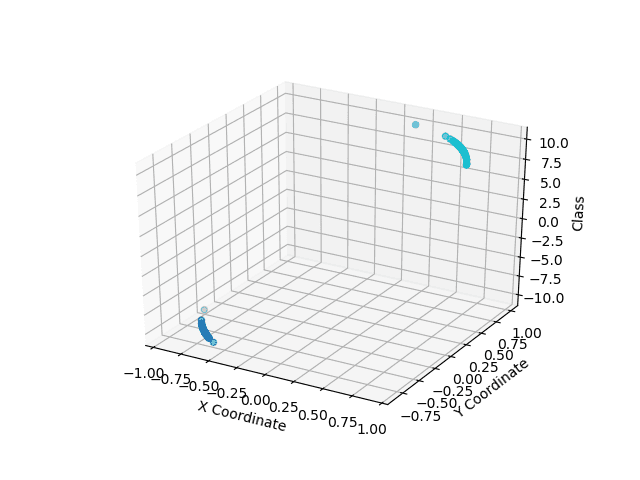
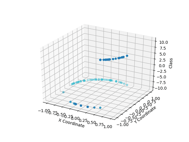
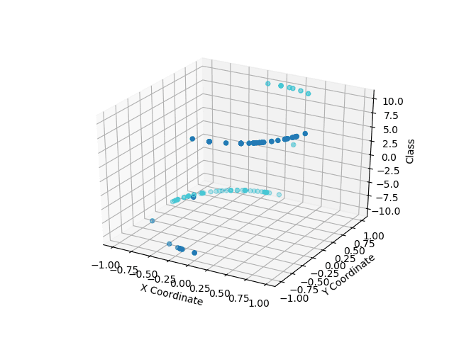
These graphs show the quantum classification results in the Z axis, with the point color representing the ground truth classes. Light blue on the top and dark blue on the bottom are correctly classified. Apparent clustering in the data before classification is due to the normalization pre-processing.
IBMQ classification Result - Linearly separable classes
Rigetti classification Result - Linearly separable classes
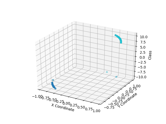
Both devices performed very well in classifying the linearly separable classes, showing that the quantum classifier can, at the very least, match the capabilities of simple classical statistics.
However, we can see some impactful differences between the two in the more challenging classes to separate. The IBM system captured an entire class with some misclassification on the dark blue class, while the Rigetti system had misclassification on both classes. Here, we see a precision-recall trade-off, with IBM providing a higher recall for a given precision and the Rigetti system reaching a more balanced precision/recall.
IBMQ classification Result - Non Linearly separable classes
Rigetti classification Result - Non Linearly separable classes
§ 4How has the state of quantum machine learning changed since 2019?
Quantum machine learning has undoubtedly grown in the past four years; one of the most exciting advancements was surprisingly an improvement in accuracy rather than efficiency: see QSVM. This project was a fantastic exploration of what is possible and some practical limitations of using a quantum computer. Some of the leading issues we faced had to do with shockingly mundane aspects of the process, like loading data into the device. Loading binary data into a quantum device is infeasible mainly due to the number of qubits required to hold the data. We followed Schuld et al. in loading our data as angles contained within parameterized gates, allowing the final measurement to provide our binary class prediction. The issue, however, is how the error rates scale with additional dimensions. Adding another dimension should, in a classical computing sense, provide more information from which we can make our prediction, resulting in higher classification accuracy. Our quantum circuit did not fare so well; adding another dimension doubled the number of gates we had to use. A doubling of the number of gates will square the overall error rate.
Consider that the probability of a given gate having an error is x, and we have n gates:
Now consider doubling the number of gates such that we have 2n Gates:
Therefore, we have squared the system's error rate as a whole.
This argument is a popular rebuttal to the hype that quantum computing brings. A common counterargument is that error rates are an "engineering" problem to solve and one that we had to deal with in the early days of classical computing. Assuming that we can reduce error rates with error-correction algorithms, Schuld et al. proposed a theoretical logarithmic speedup that does not take into account error in any way. If efficient state preparation takes polynomial time before our algorithm runs, it doesn't matter how quickly it runs, as the slowest step is still the polynomial time preparation. Evaluating quantum algorithms is like evaluating these recipes:
Recipe A
Preparation: 2 hours
Cooking 0.1 hours
or
Recipe B
Preparation 0.5 hours
Cooking 0.5 hours
You cannot only look at the cooking time; you must consider all parts of the process. Likewise, the value of Quantum algorithms cannot be observed in a vacuum. A quantum algorithm is only as good as the error correction and state preparation algorithms that they require, and even in today's age, they need to look more promising.